Exporting & visualization#
Exporting is handled by special exporting classes. These classes implement all the functionality to map the the internal representation of a pattern design in fib-o-mat to any kind of output format.
Exporting can be invoked via the via the export() method of the Sample class.
Internally, the following happens on export:
Loop over every site in the sample
Add every pattern to the exporting backend
To get started with exporting, see the examples below. Further details on exporting can be found in the extending section.
Exporting microscope readable output#
Currently, the fib-o-mat package includes only one backend to generate microscope readable/specific output. This generic backend can be used to export rasterized patterns. This backend is highly adaptiv as demonstrated below.
See the extending fib-o-mat section REF for an example how to write a custom exporting backend from scratch.
Note
Some other backends are mentioned in the documentation. These are not part of the public repository for now.
The implement SpotListBackend rasterizes all patterns. In doing so, all added sites are merged. The patterning order of the individual patterns are given by the order of adding the patterns to sites and the sites to the sample.
To illustrate the different settings of the backend, we start with a simple pattern design
from fibomat import Sample, U_, Mill, Q_
from fibomat import default_backends, shapes, raster_styles


s = Sample()
site = s.create_site(
    dim_position=((0, 0), U_('µm')), dim_fov=((5, 5), U_('µm'))
)

mill = Mill(dwell_time=Q_('1 ms'), repeats=4)

site.create_pattern(
    dim_shape=(shapes.Line((-2, -2), (2, 2)), U_('µm')),
    shape_mill=mill,
    raster_style=raster_styles.one_d.Curve(
        pitch=Q_('1 nm'),
        scan_sequence=raster_styles.ScanSequence.CONSECUTIVE
    )
)

exported = s.export(default_backends.SpotListBackend)
exported.save('file.txt')
Source: viggge/fib-o-mat/-/blob/master/examples/exporting_simple.py
This will generate a file with the following content
[Info]
length_unit = µm
time_unit = µs
fov = 3.999395954391112, 3.999395954391112
center = (-0.0003020228044439133, -0.0003020228044439133)
base_dwell_time = None
total_dwell_time = 22628000.0
number_of_points = 22628
description = None
time_stamp = 2020-11-26 11:16:31.391840

[Points]
-2.00000 -2.00000 1000
-1.99929 -1.99929 1000
-1.99859 -1.99859 1000
-1.99788 -1.99788 1000
-1.99717 -1.99717 1000
-1.99646 -1.99646 1000
-1.99576 -1.99576 1000
-1.99505 -1.99505 1000
...
This output is most likely not tremendous useful besides using it to visualize the rasterized data in the ion bam simulation tool.
Customize output format#
The SpotListBackend is highly customizable. In the following, all customization options are introduced.
All settings are passed to the backend via the export() call in the Sample class.
The following parameters can be set
save_impl: allows to pass a custom saving function which handles the writing to a file. Thereby, the file format can be set.
base_dwell_time: if set, all dwell times are divided by the base dwell time. Hence, the dwell times are expressed as integer multiples of the base dwell time.
length_unit: dwell points are converted to this unit before saving
time_unit: dwell time are converted to this unit before saving (not used ifbase_dwell_timeis given)
Now, assume, that we would like to export to a file with the layout
CUSTOMFILEFORMAT
FOV=...
DWELL=...
BEGIN_DWELL_POINTS
x1, y1, t1
...
END_DWELL_POINTS
where FOV is the needed field of view and DWELL the base dwell time. x_n and y_n are the dwell point positions given in µm and t_n dwell point multiplicands of the base dwell time (= 0.1 µs).
To use the correct lengths and time multiplicands in the exported file, we only need to add these parameters to the exporting function
exported = s.export(
    default_backends.SpotListBackend
    base_dwell_time=Q_('0.1 µs'),
    length_unit=U_('µm')
)
Finally, a custom save_impl is missing. The save save_impl function expects three parameters:
a filename, a numpy array with the dwell points and last, a dictionary which contains some useful information about the rasterized pattern and the backend’s settings. See the default implementation of the save_impl to get a complete list of available keys.
def custom_save_impl(filename: utils.PathLike, dwell_points: np.ndarray, parameters: Dict[str, Any]):
    # fov is in units of length_unit
    fov = max(parameters["fov"].width, parameters["fov"].height)

    base_dwell_time = units.scale_to(U_('µs'), parameters["base_dwell_time"])

    with open(filename, 'w') as fp:
        # first, write header data.
        fp.writelines([
            'CUSTOMFILEFORMAT\n',
            f'FOV={fov:.3f}\n',
            f'DWELL={base_dwell_time:.1f}\n',
            'BEGIN_DWELL_POINTS\n'
        ])

        # second, write dwell point data
        # dwell_points has shape (N, 3) where N is the numbre of dwell points. Each row in the array contains
        # (x, y, t_d) where x and y are the position of a spot and t_d the dwell time or dwell time multiplicand.
        # "%.5f %.5f %d" is the formatting string. See numpy doc for details on that.
        np.savetxt(fp, dwell_points, "%.5f %.5f %d")

        fp.write('END_DWELL_POINTS\n')
If added to the export function
exported = s.export(
        default_backends.SpotListBackend
        base_dwell_time=Q_('0.1 µs'),
        length_unit=U_('µm'),
        save_impl=custom_save_impl
    )

 exported.save('file.txt')
the export yields a file with content
CUSTOMFILEFORMAT
FOV=3.999
BEGIN_DWELL_POINTS
-2.00000 -2.00000 10000
-1.99929 -1.99929 10000
-1.99859 -1.99859 10000
-1.99788 -1.99788 10000
-1.99717 -1.99717 10000
-1.99646 -1.99646 10000
...
END_DWELL_POINTS
Source: viggge/fib-o-mat/-/blob/master/examples/exporting_advanced.py
Set exported sites#
The method export_multi() exports every site of site individually and returns a list containing instances of the exporting backend for every site.
from fibomat import Sample
from fibomat import default_backends

sample = Sample()

# ...

exported_sites = smaple.export_multi(default_backends.SpotListbackend)

for i, exported in enumerate(exported_sites):
    exported.save(f'file_{i}.txt')  # save txt file for each exported site.
The method export_with_description() allows to specify sites for exporting witch match a given regular expressions.
from fibomat import Sample
from fibomat import default_backends

sample = Sample()

# ...

descr_pattern = [
    'foo',    # this matches sites where the description contains 'foo', e.g. 'foo_1', 'foo', 'foobar'
    r'^bar$'  # this matches sites where the description is exactly 'bar'
]
exported_sites = sample.export_with_description(default_backends.SpotListbackend, descr_pattern=descr_pattern)

# do something with exported sites
Use https://regex101.com/ for example to test regular expressions.
Visualization#
Generating interactive plots#
fib-o-mat ships with a default plotting backend. This backend is based on the bokeh library. The backend generates an interactive html file viewable in any modern browser. This file does not depend on the fib-o-mat python package. Hence, it can be distributed and used easily without any python dependenciess.
Plots can be generated via the plot() method of the Sample class.
The plotting can be configured with the following parameters:
filename: if given, the plot is saved with the given name. Default to None.
show: if True, the plot is opened in a broser windows. Default to True.
unit: the length unit of the axes, by default µm
title: title of the plot, by defaultSample.description
hide_sites: if True,Sitess are not shown in the plot, by default False
rasterize_pitch: the pitch used to rasterize all plotting data to polylines, by defaultQ_('0.01 µm')
legend: if True, a legend with all sites as entries is shown, by default True
cycle_colors: if True, each site and all its shapes will get a different color, by default True
See the examples folder in the git repository for examples how to use the backend. At the end of the getting started guide, all features of the generated plot are explained.
To save a html file, use
s = Sample()

# ...

s.plot(filename='my_plot.html')
#or
s.plot(filename='my_plot.html', show=False, hide_sites=True, legend=False)
Warning
Only raw shapes are plotted and not newly generated shapes by patterning backends.
Annotation layer#
To add annotations to a plot, the Sample class has a add_annotation() method.
This annotation are only used on plotting and no other backend can access them.
Any pre-defined shape introduced at Geometric shapes can be used as an annotation.
The added shape can be draw filled an the color can be customized.
To define the scaling of the annotations, these must be equipped with a length unit (similar to shapes in Pattern).
The position of annotations is always to the gloabl coordinate system.
from fibomat import Sample
from fibomat.shapes import Line, Circle

s = Sample()

s.add_annotation(Line((0, 1), (1, 1)) * U_('µm'))
s.add_annotation(Circle(r=1, center=(1, 1)) * U_('µm'), filled=True, color='blue')

s.plot()
Colors must be defined in a way that bokeh can understand them (cf. bokeh doc).
Ion beam simulation#
Files exported with the default SpotList backend can be visualized with the beam_simulation tool. This tool animates the beam path and should show quantitatively the same what a real microscope would do.
The tool can can be run from the command line with
$ beam_simulation path/to/the/exported/file.txt
This works only, if the python binary directory is in the PATH variable, e.g. if a virtual environment is used.
For better visualization, the beam is shown with a tail. The animation speed can be changed manually to adapt for different dwell point densities. The dwell time of the points is ignored.
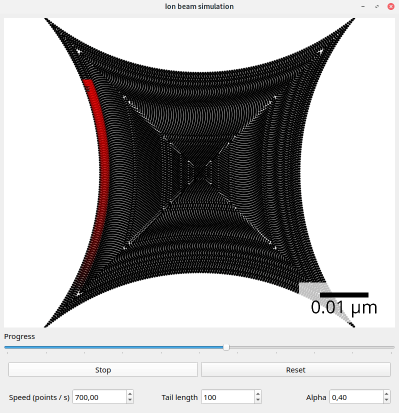
Screenshot of the beam simulation tool.#